1.Ceres官方教程-非线性最小二乘～Hello World!

翻译:http://ceres-solver.org/nnls_tutorial.html
参考:https://blog.csdn.net/wzheng92/article/details/79700911?spm=1001.2014.3001.5501

1.介绍

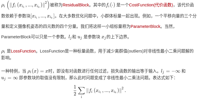
Ceres 可以解决以下形式的边界约束鲁棒化非线性最小二乘问题
    

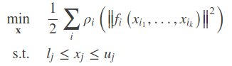
"非线性"是指代价函数为非线性函数。
 

这一表达式在工程和科学领域有非常广泛的应用。比如统计学中的曲线拟合，或者在计算机视觉中依据图像进行三维模型的构建等等。

2.Hello World!

首先，考虑寻找函数的最小值的问题。
    

这是一个微不足道的问题，其最小值位于x = 10，但这是一个很好的起点，可以说明使用Ceres解决问题的基础知识。
第一步是编写一个函子来评估这个函数f(x) = 10 - x

// 构建代价函数，重载()符号
struct CostFunctor {
   template <typename T>
   bool operator()(const T* const x, T* residual) const {
     residual[0] = 10.0 - x[0];
     return true;
   }
};

这里需要注意的重要一点是，operator()是一个模板化方法，它假定其所有输入和输出都是某种类型T。这里使用模板允许Ceres调用CostFunctor::operator()，当只需要残差值时使用T=double，当需要雅可比矩阵时使用特殊类型T=Jet。
一旦我们有了计算残差函数的方法，现在是时候用它来构造一个非线性最小二乘问题并让Ceres来解决它了。

完整的代码在ceres-solver-1.14.0/examples/helloworld.cc中

#include "ceres/ceres.h"
#include "glog/logging.h"

using ceres::AutoDiffCostFunction;
using ceres::CostFunction;
using ceres::Problem;
using ceres::Solver;
using ceres::Solve;

// A templated cost functor that implements the residual r = 10 -
// x. The method operator() is templated so that we can then use an
// automatic differentiation wrapper around it to generate its
// derivatives.
// 第一部分：构建代价函数，重载()符号，仿函数的小技巧
struct CostFunctor {
  template <typename T> bool operator()(const T* const x, T* residual) const {
    residual[0] = 10.0 - x[0];
    return true;
  }
};

int main(int argc, char** argv) {
  google::InitGoogleLogging(argv[0]);

  // The variable to solve for with its initial value. It will be
  // mutated in place by the solver.
  // 设置寻优参数x的初始值，为0.5
  double x = 0.5;
  const double initial_x = x;

  // Build the problem.
  Problem problem;

  // Set up the only cost function (also known as residual). This uses
  // auto-differentiation to obtain the derivative (jacobian).
  // 第二部分：构建寻优问题
  CostFunction* cost_function =
  // 使用自动求导，将之前的代价函数结构体传入，第一个1是输出维度，即残差的维度，第二个1是输入维度，即待寻优参数x的维度。
      new AutoDiffCostFunction<CostFunctor, 1, 1>(new CostFunctor);
  // 向问题中添加残差项，本问题比较简单，添加一个就行。
  problem.AddResidualBlock(cost_function, NULL, &x);

  // Run the solver!
  // 第三部分： 配置并运行求解器
  Solver::Options options;
  options.minimizer_progress_to_stdout = true;
  // 注意：下面这两行是新加的，因为默认编译的ceres不支持SPARSE_NORMAL_CHOLESKY
  options.linear_solver_type = ceres::DENSE_QR;
//   options.sparse_linear_algebra_library_type = ceres::NO_SPARSE;
  Solver::Summary summary; // 优化信息
  Solve(options, &problem, &summary);// 求解!!!

  std::cout << summary.BriefReport() << "n"; // 输出优化的简要信息

  std::cout << "initial x : " << initial_x << ", "
            << "result x : " << x << "n";
  return 0;
}

运行结果

iter      cost      cost_change  |gradient|   |step|    tr_ratio  tr_radius  ls_iter  iter_time  total_time
   0  4.512500e+01    0.00e+00    9.50e+00   0.00e+00   0.00e+00  1.00e+04        0    2.84e-05    2.52e-04
   1  4.511598e-07    4.51e+01    9.50e-04   9.50e+00   1.00e+00  3.00e+04        1    3.36e-05    3.15e-04
   2  5.012552e-16    4.51e-07    3.17e-08   9.50e-04   1.00e+00  9.00e+04        1    2.11e-05    3.62e-04
trust_region_minimizer.cc:687 Terminating: Parameter tolerance reached. Relative step_norm: 3.166209e-09 <= 1.000000e-08.
Ceres Solver Report: Iterations: 3, Initial cost: 4.512500e+01, Final cost: 5.012552e-16, Termination: CONVERGENCE
initial x : 0.5, result x : 10

初始值为0.5，最终通过3次循环之后到达最优解10。其实本例是一个线性问题，因为
f(x)=10−x是一个线性函数，但是Ceres仍然可以应用。对于Ceres解非线性应用的流程和具体配置将在后续的教程中给出。

代码解析: 1.构建代价函数

使用了仿函数，即在CostFunctor结构体内，对()操作符进行了重载，这样使该结构体的一个实例就能具有类似一个函数的性质，在代码编写过程中就能当做一个函数一样来使用。

仿函数: https://www.cnblogs.com/vivian187/p/15329482.html
代价函数:

代码解析: 2.配置问题并求解问题

注意：相对于源代码，这里新添加了

options.linear_solver_type = ceres::DENSE_QR;

原因：因为ceres-solver-1.14.0的CMakeLists.txt中的默认配置，导致SuiteSparse, CXSparse等不可用。因此运行时会出现如下问题

solver.cc:531 Terminating: Can't use SPARSE_NORMAL_CHOLESKY with SUITESPARSE because SuiteSparse was not enabled when Ceres was built.

线性求解器的类型，用于计算Levenberg-Marquardt算法每次迭代中线性最小二乘问题的解。 如果编译Ceres时加入了SuiteSparse或CXSparse或Eigen的稀疏Cholesky分解选项，则默认为SPARSE_NORMAL_CHOLESKY，否则为DENSE_QR。

DENSE_QR: 对于较小的问题(几百个参数和几千个残差)，相对稠密的Jacobians，DENSE_QR 是一个选择。
DENSE_NORMAL_CHOLESKY & SPARSE_NORMAL_CHOLESKY: 大型非线性最小二乘问题通常是稀疏的。在这种情况下，使用稠密的QR分解是低效的。